Simulating Brownian Motion with Dynamic Visualization

The project simulated random walk physics based on normal distribution, leveraging numerical methods and real-time plotting.

Introduction

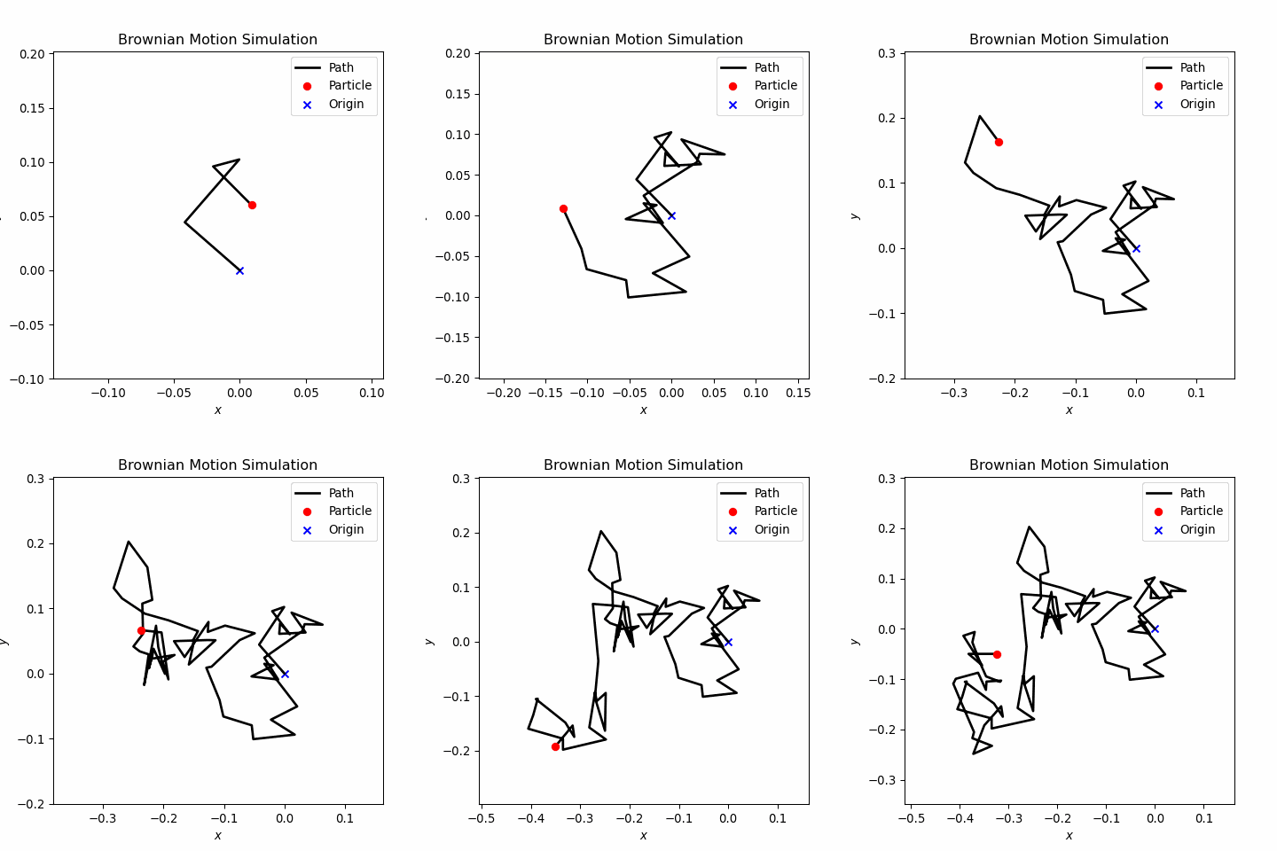
Brownian motion, also known as a random walk, describes the erratic and random movement of particles in a fluid due to collisions with molecules. This project simulates the 2D Brownian motion of a particle using a random walk model based on a normal distribution. The simulation leverages numerical methods and visualizes the path dynamically, offering insights into the physics of stochastic processes.

Code

import numpy as np
import matplotlib.pyplot as plt
from matplotlib.animation import FuncAnimation, PillowWriter
from IPython.display import display, HTML

# Parameters
N = 100  # Number of steps
delta = 0.4  # Random distribution tuner; sigma = (delta**2)*dt
dt = 0.2  # Time step
x, y = [0], [0]  # Initial positions

# Create figure and axes
fig, ax = plt.subplots(figsize=(5, 5), dpi=100)
path_line, = ax.plot([], [], "k-", lw=2, label="Path")
particle, = ax.plot([], [], "ro", label="Particle")
ax.scatter(0, 0, c="blue", marker="x", label="Origin")  # Origin
ax.set_xlim(-1, 1)
ax.set_ylim(-1, 1)
ax.set_xlabel(r"$x$")
ax.set_ylabel(r"$y$")
ax.set_title("Brownian Motion Simulation")
ax.legend()

# Update function for animation
def update(frame):
    global x, y
    x_new = x[-1] + np.random.normal(loc=0, scale=(delta**2) * dt)
    y_new = y[-1] + np.random.normal(loc=0, scale=(delta**2) * dt)
    x.append(x_new)
    y.append(y_new)
    
    path_line.set_data(x, y)
    particle.set_data(x[-1], y[-1])
    
    # Adjust axis limits dynamically
    ax.set_xlim(min(x) - 0.1, max(x) + 0.1)
    ax.set_ylim(min(y) - 0.1, max(y) + 0.1)
    return path_line, particle

# Create the animation
ani = FuncAnimation(fig, update, frames=N, interval=100, blit=True)

# Save the animation as a GIF
gif_path = "brownian_motion.gif"
ani.save(gif_path, writer=PillowWriter(fps=10))

# Display the GIF inline
display(HTML(f'<img src="{gif_path}" alt="Brownian Motion Simulation">'))

Output

Animated simulation of a two-dimensional Brownian motion, showcasing the random path of a particle generated using a normal distribution for step displacements.